Phase Unwrapping in C#

TL;DR

Phase unwrapping is the process of adding multiples of \( 2\pi \) to an n-dimensional “wrapped” phase distribution to recreate a continuous curve. Phase unwrapping in two-dimensions (i.e. over an image) is an algorithmic requirement for many imaging modalities, including many interferometric techniques, Doppler Optical Coherence Tomography (OCT), height correction in Spatial Frequency Domain Imaging (SFDI), and phase analysis in Magnetic Resonance Imaging (MRI). A variety of phase unwrapping algorithms have been developed, packaged, and distributed for public use, but these algorithms are typically implemented in either Python or MATLAB, making it difficult for production applications in other languages to employ the developed algorithms. This post (i) describes the use of phase unwrapping for Phase Profilometry, to illustrate a use-case for the algorithm, and (ii) introduces an open-source C# implementation of a reliability-guided phase unwrapping algorithm. The implementation is published on Nuget here.

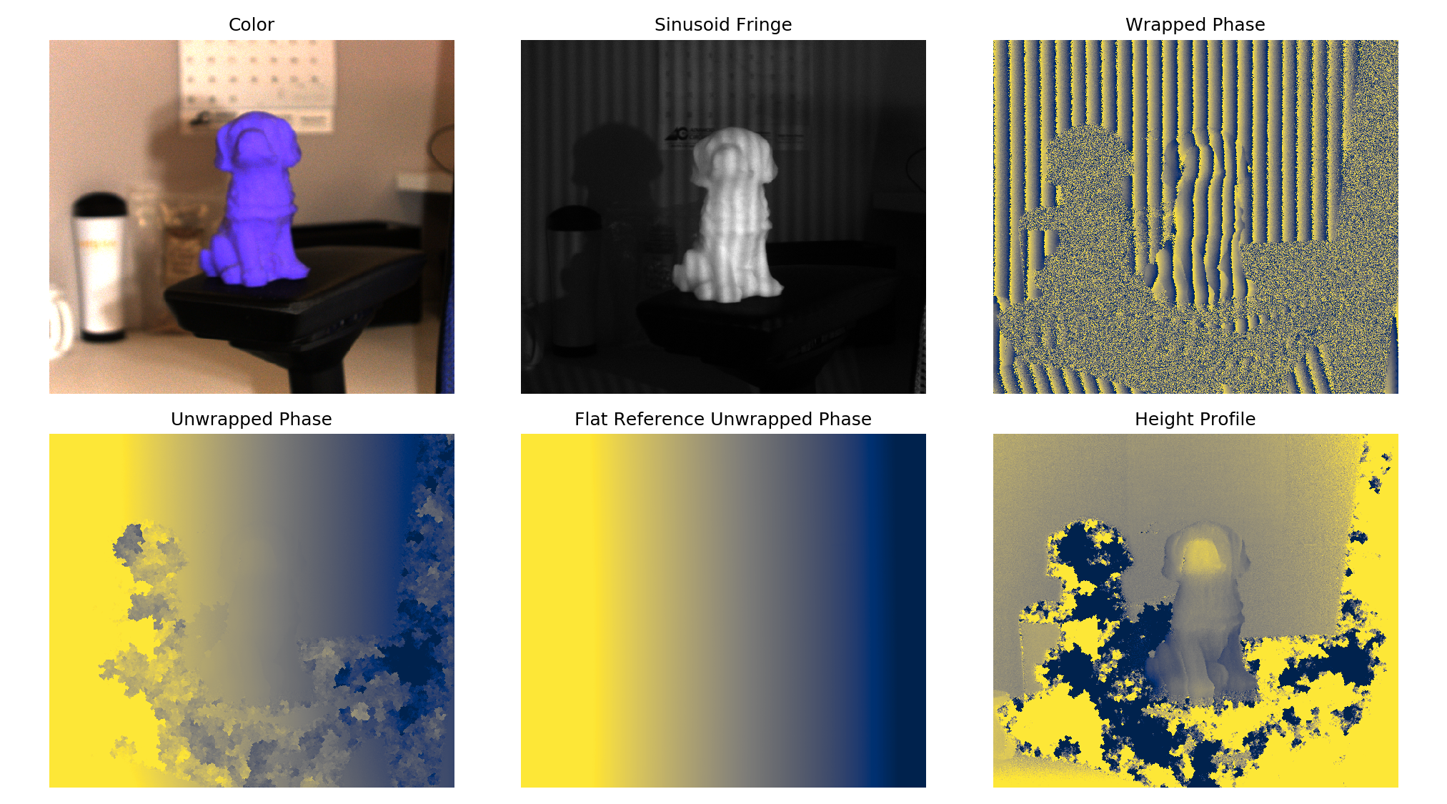Figure 1: Example of Phase Profilometry applied to a 3D-printed figurine of a puppy. The algorithm’s steps move from top left to bottom right in the figure, starting from the fringe images through to the Height Profile image. This final map is proportional to the “height” of the target’s profile (note that the dog’s snout is the “highest” part, i.e., closest to the camera).

Phase Shifting Profilometry

For many applications, including manufacturing quality assurance, computer aided design, and augmented reality, the 3 dimensional surface profile of an arbitrary object must be measured and digitized. The process of measuring the surface profile of a target is known as Profilometry. One of the more common (and simple) profilometry techniques is Phase Shifting Profilometry (PSP), in which a series of 3 structured light images (e.g., the “Sinusoid Fringe” image shown in Figure 1) are projected onto the target. In PSP, these projected images contain intensity modulations following a sine curve in 1 dimension. By “shifting” the phase offset of the projected pattern along the axis of modulation, the Phase Distribution of the tissue can be accurately captured. See the below equation for computing the wrapped phase distribution (\(\phi^{wrapped} \)) from the captured reflected intensity, where \(I_0\), \(I_1\), and \(I_2\) are the intensities of the captured images considering 0, 120, and 240 degree phase offset projections, respectively. All the variables defined are images, i.e., they vary along x and y.

$$ \tag{1} \phi^{wrapped} = arctan({\sqrt{3}\frac{I_1 - I_2}{2I_0 - I_1 - I_2}}) $$

• Note that the arctan in the above formula is the 4-quadrant tangent, commonly called Atan2

The reflected phase contains information about how the target has warped the projected light patterns. However, there are two problems with this approach - the first is that we don’t know how a flat surface would impact the phase distribution, and the second is that the “wrapped phase” must be unwrapped before it can be used to extract surface profile.

Normalization to Flat Reference

This problem can be easily addressed by capturing the phase of a flat surface, and then normalizing the phase of the target by this “flat surface” phase, which we’ll call the “Reference Phase”, or \(\phi_0\) . Quite conveniently, observed phase differences are proportional to the “height” (\(Z\)) differences between the flat surface (reference) and the target, according to a relationship that can be derived from the triangulation geometry between the camera, projector, and target (Fig. 2).

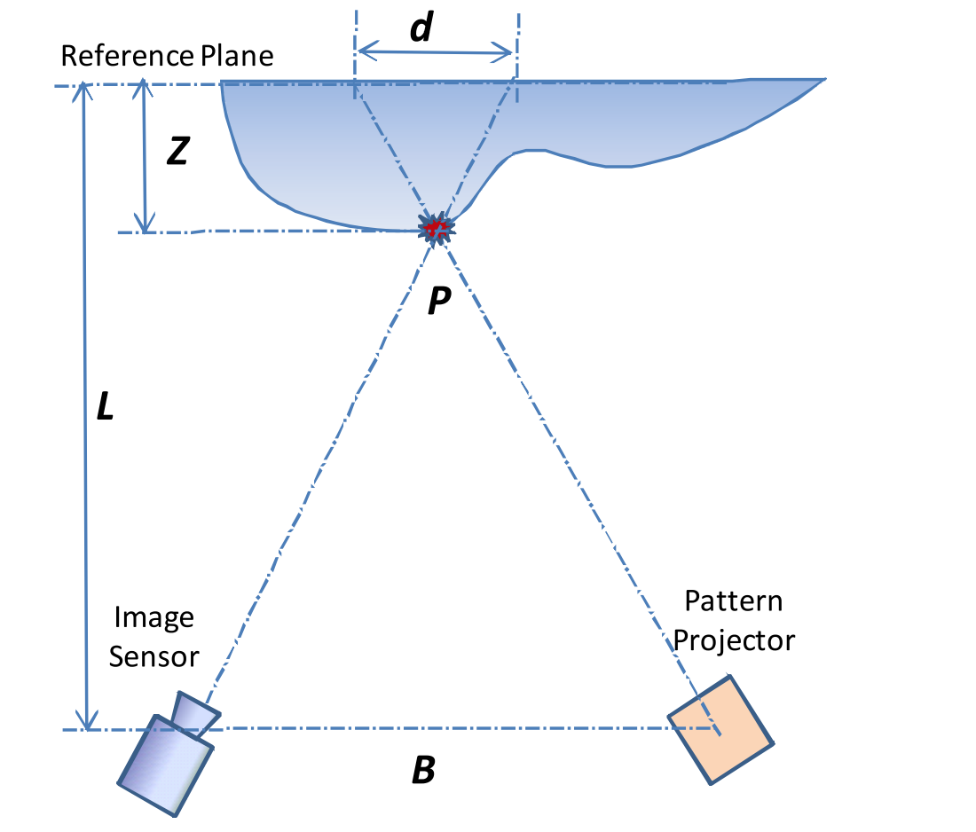Figure 2: Example of the triangulation geometry and the extraction of the pixelwise height from an example target surface. The Reference Plane shown in the image is the plane which is imaged during the normalization step, which results in the Reference Phase, or \(\phi_0\). Figure copied from Geng 2010.

The exact coefficient relating the relative phase to the height can be computed theoretically from the known projection, projector, and camera geometries, but can much more easily be approximated via the following equation, from Ch.8 in Geng 2010:

$$ \tag{2} Z \approxeq \frac{L}{B} * d \propto \frac{L}{B}(\phi - \phi_0) $$

With this formula, acquiring an appropriate reference phase will solve the first of the challenges in phase profilometry. The second problem with using the phase to extract target height is evident in the formula presented for computing \(\phi^{wrapped}\). See if you can find it before you read the below paragraph.

Phase Unwrapping

The second problem with Eqn. (1) is that it computes the wrapped phase (\(\phi^{wrapped}\)) rather than the absolute phase (\(\phi\)). The phase output by Eqn. (1) is called wrapped because the computation is enclosed by the arctangent function, which will always return a value within the range \((-\pi, \pi)\). However, assuming the image contains multiple projection fringes of the fringe projection pattern (it typically does; see e.g. fringe image in Figure 1), the full range of the phase will be much larger. Because Eqn. (1) constrains the output phase to within the range of \((-\pi, \pi )\), we call this output the Wrapped Phase. To restore the wrapped phase image to a close approximation of the absolute phase, a 2D Phase Unwrapping algorithm is typically employed. A phase unwrapping algorithm describes the a 2D map indicating how many increments of \(2\pi\) to add to / subtract from each pixel in order to recreate a continuous phase, s.t., at each pixel

$$ \tag{3} \phi \approxeq \phi^{wrapped} + 2k\pi $$

where \( k \in \mathbb{Z} \). A linetrace illustrating the wrapped phase values (\( \phi^{wrapped}\)), the unwrapping interval added (\(2k\pi\)), and the unwrapped phase (\(\phi\)) for a series of pixels along the center of the image is shown in Figure 3 below.

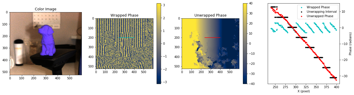Figure 3: Example of the effects of 2D phase unwrapping shown via images and lineplot. Note that the phase unwrapping adds successive intervals of \(2\pi\) to the unwrapped phase to recreate a contiguous phase (unwrapped phase). Thus, at each point, the wrapped phase plus the unwrapping interval yields the unwrapped phase (see Eqn. (3)).

Additionally, because both the reference phase (\(\phi_0\)) and the target phase (\(\phi\)) are computed via Eqn. (1) above, both phases must be unwrapped before Eqn. (2) can be applied to extract the target height.

Putting It All Together

By addressing the two main challenges with Eqn. (1), we can now describe how to extract target height from phase in PSP. See the below instructions describing how to perform PSP:

Reference Acquisition

1. Acquire 3 images of 120-degree phase-shifted sinusoidal patterns projected onto a Flat Reference Surface
2. Extract the wrapped phase of the reference fringe images according to Eqn. (1) => \(\phi_0^{wrapped}\)
3. Unwrap the flat reference phase using a phase unwrapping algorithm. Ensure the unwrapped phase is 0 at a defined point by subtracting the phase at this point from the each point in the image => \(\phi_0\)

Target Acquisition

4. Acquire 3 images of 120-degree phase-shifted sinusoidal patterns projected onto a Target Surface
5. Extract the wrapped phase of the target fringe images according to Eqn. (1) => \(\phi^{wrapped}\)
6. Unwrap the target phase using a phase unwrapping algorithm. Ensure the unwrapped phase is 0 at defined center-point by subtracting the phase at this point from the each point in the image => \(\phi\)
7. Compute the target height via the relationship shown in Eqn. (3). The output of the \(\phi - \phi_0\) will be proportional to the height of the tissue.

• The exact height of the surface profile (in desired height units) can be defined by acquiring multiple phase images of the flat surface at known heights, or by computing from a known geometry.
• The defined point for ensuring the phases are not uniformly offset is often taken as the center point of the image.

In Figure 4 below, we have shown a few intermediate outputs of the PSP process for different target types:

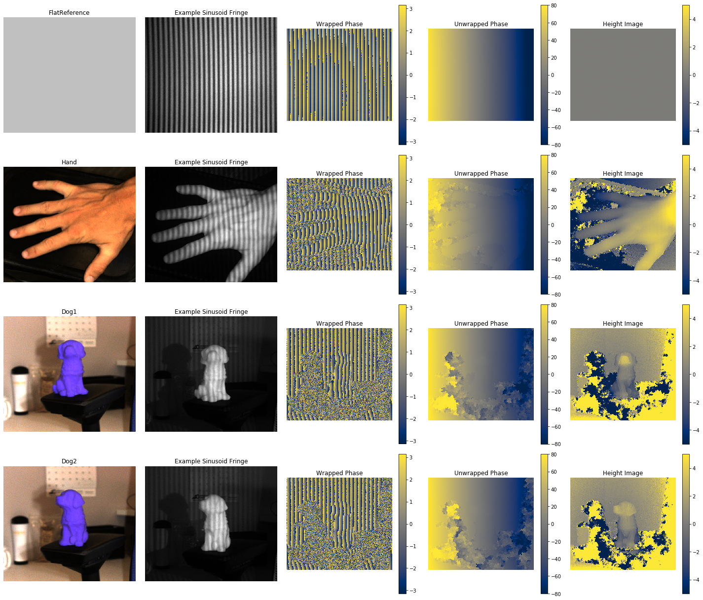Figure 4: Examples of the images of 4 different targets at various stages of the PSP algorithm. Note that the reference phase was used to compute the Height Images for each of the FlatReference, Dog1, Dog2, and Hand targets.

In conclusion, PSP is a valid and useful method for measuring the surface profile of an arbitrary target. The C# implementation of the reliability-guided phase unwrapping algorithm, published on Nuget here, will allow production applications written in the .NET ecosystem to easily unwrap “wrapped” phase signals.

Repeatability

All code needed to create the examples shown in this report is available by downloading the zipped file here. Figures in the report were generated in a Jupyter Notebook, also included in the zip file. The CAD model (STL file) of the 3D printed puppy shown in the figures is available at this website and can be downloaded here.

Further Recommendations for Computer Vision in .NET

There is an excellent .NET wrapper for the common computer vision library OpenCV called OpenCVSharp, that provides easy access to most of the basic computer vision necessities (image convolution) and is accessible via the Nuget package manager in C#. I highly recommend starting with this library if you are creating a project requiring computer vision functionality in C#. Also, for an alternative phase unwrapping algorithm, there is a phase unwrapping module in the “OpenCV Contrib” package; however, it is not clear when contributions packages like these will make it into the main OpenCV, and further into the OpenCVSharp package mentioned previously.