on
A Modern Template for Engineering Assignments
TL;DR: Using a combination of Jupyter Lab/Notebooks and the Python package Sympy as a standard for the completion and submission of engineering homework assignments can: (1) Dramatically improve the readability of mathematics, making assignments more valuable for reference and easier to grade, (2) Improve time-efficiency for students through code reuse and symbol-value substitution in defined equations, and (3) Provide a method to easily reference external media and build a rich document to explore engineering solutions quantitatively and graphically. Live example notebook.
An Argument for Improving Submission Templates
Before going into details about this approach, I wanted to address that I’ve earned my Bachelor of Science and am completing my Master of Science in Mechanical Engineering, which has provided much of the foundation and motivation for this post. I have considerable experience completing weekly assignments, which are the norm for engineering courses in the first few years of undergraduate education. I don’t think there is anything flawed with this teaching/learning approach, but I believe the typical submission media, specifically the paper-based submission of work, is a reflection of antiquated norms in engineering. How much easier would the process be for everyone involved if the assignments were submitted digitally? How much more valuable and usable would the assignments be when, 3 years down the road as a graduate researcher, the student needs to recall content from their Introduction to Fluid Mechanics course? Given the choice between sorting through stacks of paper files, assuming I happened to swing by the TA’s office to pick up the graded assignment, and searching through the Fluid_Mechanics folder on my laptop, I would take the latter every time. Additionally, if you’re like me, your paper assignments are a sparsely-connected graph of arbitrarily placed equations interspersed with scribbled-out nonsense and logic jumps justified by statements like “derived in class”. Perhaps most damning, my paper assignments frequently lacked reference to the homework problems themselves, at best containing a header like 2.12, letting me know the question is number 12 in chapter 2 of a book somewhere.
In addition to the cost to the student, I don’t know how or why Teaching Assistants (TAs) handle the poor input they receive. In other engineering settings, data transfer via handwritten paper is a ticket for a stare that asks Is this a joke?. Imagine if your manager requested a report about a topic and you handed him some some notes scrawled with your best mechanical pencil. He’d look at you like you were a third grader.
Most engineers have the good sense not to take the paper-and-pencil approach, so they instead break out their favorite MS Word software, and god help them if they need to write equations in the report, because Word’s editor has about the same user-friendliness as an F-35. It’s a shame, because better tools exist for formatting equations, but they frequently aren’t taught in school. Regardless, speaking to all of the TAs out there, wouldn’t your jobs be much easier and more straightforward if students’ work was digitally accessible and presented in a logical, sequential manner?
Before diving in, a minor concession: there do, in fact, exist many digital systems in place for homework submission and uploads (think Canvas or similar software). For our intents and purposes we will consider these similar to paper submission, as they provide little more than a means of uploading paper documents as PDFs for grading. It is apparent the practice of pen-and-paper submissions in our institution and many others is deeply ingrained. What follows is a case for improvement.
The Path to Improvement
From my perspective, it’s clear from both ends that something needs to change in the way engineering homework assignments are submitted. The good news is that this change can come from different groups and in different ways: (1) Individual students could adopt a digital approach to their assignments and negotiate with their TAs to ensure this improved format is acceptable, (2) TAs could require a digital format for all submissions, and could go beyond this to require a standardized digital format, or (3) Faculty could recognize the deficiencies in the current model and advocate for digital submissions. My point is, if you are involved in engineering instruction (i.e., a student, TA, or professor), you can advocate for digital revolution to the assignment submission system.
You may still have some questions about the proposed digital model, and I’ve tried to address some in the below Q/A. I’m happy to have further discussion in the comments section.
- Won’t requiring digital submissions make it harder on students?
- Not at all. I believe it will actually make it easier on them, by forcing them to learn and follow a logical, sequential, algorithmic way of thinking. As I will demonstrate later, if implemented correctly it can also teach students some valuable skills and ideas, such as elementary programming, function modularity, and the importance of considering the recipient of their work.
- Won’t digital submissions encourage cheating?
- Possibly. But the reality is that assignments encourage cheating. And while the ease of software transmission might make cheating apparently easier, tools exist that can identify cheating in digital submissions. These tools could render cheating detection more effective in digital than print and help to combat this potential problem.
- Will this require me to learn some new piece of software?
- Most likely, yes. But the cost of learning will be overshadowed by the value of the solution, both in time savings and benefits to the students and graders.
- What format should these digital submissions take?
- Read on : )
A New Digital Homework Template
Like the standard paper-and-pencil template for assignment submission, a digital template should:
- Minimize time expense for documenting assignments after completion
- Permit simple commenting by graders
- Be encompassed in a low-overhead solution, both in cost and resource requirements
- Allow a wide variety of scientific symbols and operation
In addition to these capabilities, an effective digital template should:
- Encourage reuse of simple mathematical operations and problem sub-steps
- Allow inclusion of simple reference to internet resources and other media
- Be rapidly extensible with respect to graphing and plotting
- Enforce sequential order of clear mathematical operations
- Require the document to be explicity legible and easily accessible, shareable, and store-able
To fulfill these requirements, I propose a combination of the Jupyter Lab/Notebooks framework with the Sympy Python package for symbolic mathematical computation. These two powerful packages collaborate to provide an elegant solution to the requirements listed above.
Briefly, Jupyter Lab, a recent iteration of the popular Jupyter Notebooks, permits modular code and documentation through a linear set of cells which can be denoted as markdown or code cells. Cells can be run individually or grouped and run sequentially, with the variable/class/function namespaces persisting across cells in both cases. When run, markdown cells will render the enclosed content in the space directly beneath the cell (see below).
print('Hello World')
Hello World
This proximity between source code and output encourages rapid understanding and simplifies finding bugs. These code cells execute the source code in a Python ‘kernel’ – a configurable construct combining the Python interpreter, a Python environment with environment libraries and modules, and the current variable/function/class namespaces – and render output in the space below the cell (see below).
# Output examples in Jupyter
from pylab import *
import numpy as np
from IPython.display import display, Markdown, Latex
# You can print normally
print("Hello Everybody ")

# You can plot
x_values = np.linspace(0,10, 100)
plot(x_values,np.sin(x_values) , 'b', label = "Statistics aren't real")
plot(x_values,np.cos(2*x_values) , '4r', label = 'Data is Fake')
legend()
show()

# You can output equations in Latex
display(Markdown('$a^2 = b^2+c^3$'))

# You can insert comments in red easily
display(Markdown("<font color='red'>The Pythagorean theorem equation is incorrect</font>"))
# You can write Markdown
display(Markdown('[*Click*](https://google.com) `for` the **answer to Life**'))
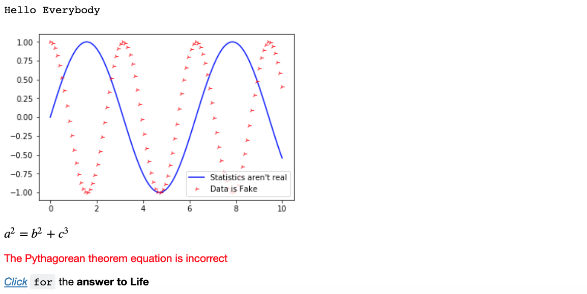
As shown, this code output can consist of an arbitrary combination of print() statements, plots to display relationships, markdown output (to include external images, for example), LaTeX to display equations, and any other type of output you want to render via HTML or similar – Recently, new interactive functionality was introduced to Jupyter, permitting Javascript embedding into Jupyter notebooks (example here). This rich cell -> output model is perfectly adaptable to the homework assignment standard, where independent problems are completed and documented in sequential order. Additionally, the digital nature of cells encourages further understanding of the problem through plotting and graphical analysis, documentation of resources for solving the problem, and simple visualization of the problem solution.
Why Sympy?
Although I expect a variety of packages would eventually be used in these digital assignments (numpy, matplotlib, pillow, and pandas come to mind), I wanted to bring attention to the Sympy package for its ability to operate on symbolic variables abstracted from numerical assignment. The idea of symbolic logic, i.e., using symbols to represent properties and operations, is fundamental to mathematics theory. Moreover, the derivation and production of closed-form, as opposed to numerical, solutions to mathematical problems is vital for their general applicability and the deeper understanding of the problem they require. Finally, the ability to produce a symbolic representation for a solution indicates a more complete conceptualization of the problem space than the corresponding specific solution (see examples below).
Specific form: 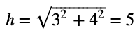
- Indicates nothing about constituents of h, only accurate for specific problem values
General form/Closed-form: 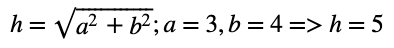
- Describes relationship between h and constituents, allowing for extensibility with similar problems
I agree that in some cases, for example when the goal of the assignment is to produce derivatives, limits, and integrals, it is unwise to allow students to explain their answer solely through Sympy code. However, I am making this argument principally for engineering rather than mathematics homework, and in engineering assignments the goal is typically understanding and applying equations to the problem system rather than derivation of the underlying mathematics. In these cases, Sympy can be a valuable tool to allow the student to focus attention and effort on the concepts that the course seeks to teach. See the examples below for ways in which Sympy can simultaneously benefit the learning experience and help to document it more effectively.
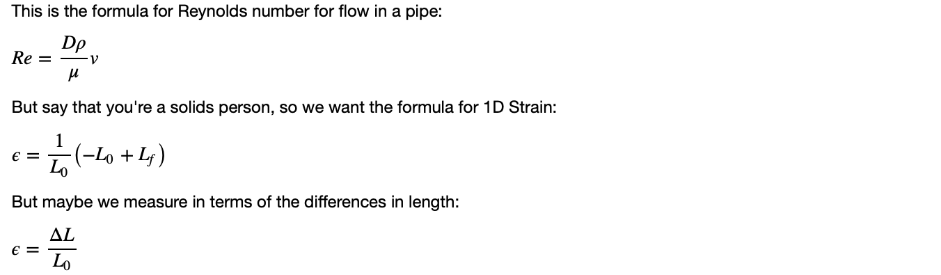
First, Sympy allows us to define equations that use symbolic variables, which will allow us to operate on them later. Additionally, Sympy allows easy rendering of these symbolic expressions, via Latex, to help users document their analysis process.
from sympy import *
from IPython.display import display, Math, Latex, Markdown

init_printing()

# Example equation for Reynolds number of flow in a pipe
Re= symbols('Re') # Reynolds number symbol
density = symbols('rho') # Density
velo = symbols('v') # Velocity
D = symbols('D') # Diameter
visc = symbols('mu') # Viscosity
Reynolds = (density*velo*D)/(visc) # Re formula

display(Markdown('This is the formula for Reynolds number for flow in a pipe: '))
display(Eq(Re,Reynolds))# this prints out the equation
display(Markdown("But say that you're a solids person, so we want the formula for 1D Strain:"))
Lf = symbols('L_f') # Final length
L0 = symbols('L_0') # Initial length
epsilon = symbols('epsilon') # Strain symbol
Strain = (Lf-L0)/L0 # Strain formula
display(Eq(epsilon, Strain))
display(Markdown('But maybe we measure in terms of the differences in length:'))
delta_L = symbols('\\Delta{L}') # Difference in length
Strain_alt = (delta_L)/l0 # Strain formula
display(Eq(epsilon, Strain_alt))
Sympy encourages evaluation of symbolic expressions via the substitute, or subs(), method, which takes arguments mapping scalar values to the symbols in a Sympy symbolic expression. This capacity makes it easy to evaluate an equation in a single additional line of code, if given values for a function:
# Sympy Subs example
display(Eq(epsilon, Strain))
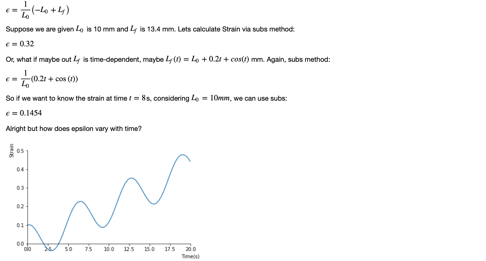
display(Markdown('Suppose we are given $L_0$ is 10 mm and $L_f$ is 13.4 mm. Lets calculate Strain via subs method:'))
strain_calc = Strain.subs({L0:10, Lf:13.2}) # Use the .subs() method to plug in arguments
display(Eq(epsilon, strain_calc))
display(Markdown('Or, what if maybe out $L_f$ depends on time, say $L_f(t) = L_0+0.2t+cos(t)$ mm. Subs method:'))
t = symbols('t') # Define the time symbol
Lf_time = L0+0.2*t+cos(t) # Define the LF_time expression
time_Strain = Strain.subs(Lf,Lf_time) # substitute Lf as a function of time into Strain
display(Eq(epsilon, time_Strain))
display(Markdown("So if we want to know the strain at time $t = 8$s, considering $L_0 = 10 mm$, we can use subs:"))
display(Eq(epsilon, round(N(time_Strain.subs({L0:10, t:8})),4))) # Display the subs result to 4 decimal places
display(Markdown('Alright but how does epsilon vary with time?'))
plot(time_Strain.subs({L0:10}), (t, 0, 20), ylabel='Strain', xlabel = 'Time(s)') # Plot Strain for t:(0,20)
Additionally, Sympy will easily compute integrals, derivatives, and other typical mathematical operations.
# Sympy for Integrals and Derivatives
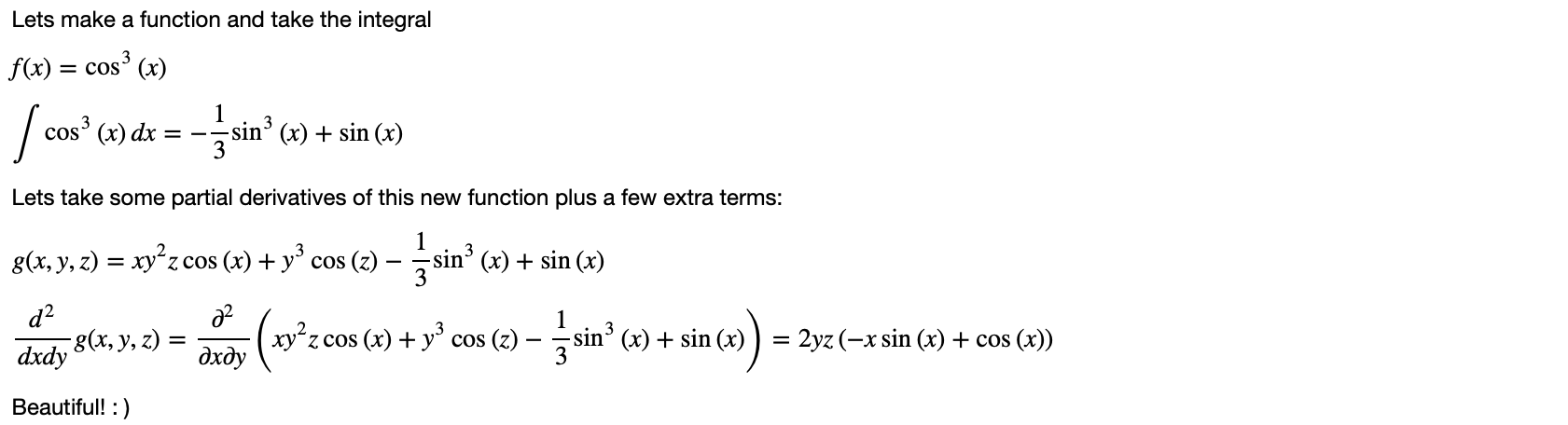
display(Markdown('Lets make a function and take the integral'))
x = symbols('x') # Define our symbols
y = symbols('y')
z = symbols('z')
func = cos(x)**3 # create our function to integrate
display(Eq(symbols('f(x)'), func))
int_func = integrate(func, x) # This is the line that actually performs the integral w.r.t x
display(Eq(Integral(func,x),int_func))
display(Markdown('Lets take some partial derivatives of this new function plus a few extra terms:'))
g_func = int_func + cos(z)*y**3 + x*z*y**2*cos(x) # Create our new function g
display(Eq(Symbol('g(x,y,z)'), g_func)) # Display the function
der_func = diff(g_func, x,y) # Take the derivative w.r.t x, then y
display(Eq(Eq(Derivative(Symbol('g(x,y,z)'),x,y),Derivative(g_func, x, y)), der_func)) # Output the Equalities
display(Markdown('Beautiful! : )'))
Sympy has many other capabilities and uses, and I encourage all interested parties to explore the documentation on their website.
Closing Remarks
I hope that this article has inspired you to reconsider your approach to engineering assignment documentation and to take an honest look at the flaws in the current system. The combined Jupyter with Sympy approach may not be perfect, but I believe it is far superior to the existing methodology. If you would like to try it out for yourself, I encourage you to experiment with the examples listed on this page, which are graciously hosted by Kyso.io at this address. For further examples of Sympy used for documentation of mathematical derivations in a Jupyter Notebook, see the polarization calculus project here. Finally, if you would like to experiment further, the remark below describes installation instructions for these two softwares.
Remark: Jupyter Lab installation will depend on an existing installation for a python interpreter and environment. These can be downloaded in a lightweight package, or in a more robust and extensible framework and library collection. Once a python interpreter and pip environment have been installed, Jupyter and sympy can be installed via the following commands in Terminal (for Unix derivatives):
pip install jupyterlab, then pip install sympy. Then, Jupyter lab can be run via the command: jupyter lab
Alternatively, on Windows, you can use python3 pip install jupyterlab, thenpython3 pip install sympy, and run Jupyter via jupyter lab.
- In Windows, depending on the python installation, sometimes the system cant find the python interpreter. In that case, see this page.